

-02")
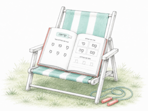
Preventing the Summer Slide
Small efforts, big impacts We know how quickly children grow when learning is consistent—and how quickly skills can fade when routines disappear for months. The “Summer Slide” is real. Children can lose foundational academic skills, and even social and emotional progress, over the break. For some, September feels less like a continuation and more like starting all over again. A few intentional moments each week throughout the summer can help reinforce and protect the skills students worked hard to master during the year. That said, summer was never meant to be a third semester. Young children still need rest, play, family time, and freedom—and the goal isn’t to push them toward new skills. It’s simply to preserve what they already know. The Balance According to one of Torah Umesorah’s leading Intervention Specialists, assigning summer homework three times a week is sufficient for maintaining students’ progress. The assignments don’t need to


One Response
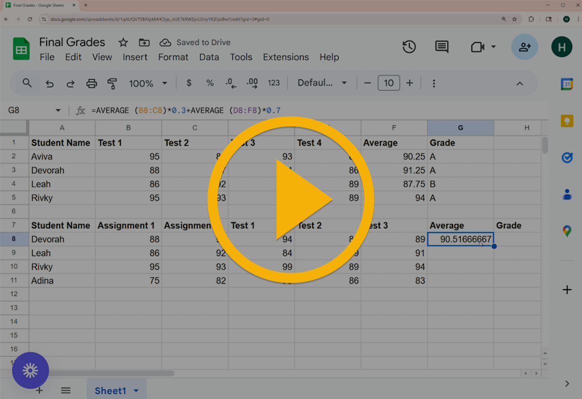
This was super helpful! I never was able to figure out how to use a spreadsheet to help calculate their final grades when tests, classwork, homework, and behavior were each counted towards different percentages of their grades. Looking forward to putting this to use and grading will be a breeze! Thank you so much!